Chapter 6 Complex Experiments
Gupta & Rickard (2022) conducted an experiment to investigate the impact of on-task trial time and break time on participants’ fatigue levels during a motor sequence task. In this task, participants repeatedly typed the sequence 4-1-3-2-4. They manipulated two independent variables: break time (10 s or 30 s) and trial time (10 s or 30 s). The dependent measure was the reaction time per keypress. Their findings indicated that both variables independently influenced reaction time, with longer breaks and shorter trials resulting in quicker reaction times. This straightforward 2x2 design is commonly used by experimental psychologists, allowing them to manipulate two independent variables, such as break time and trial time, at two levels (e.g., 10 s or 30 s) and obtain clear and interpretable results.
So far, we’ve focused on simple research designs focusing on single variables or the relationship between two variables, the experiment conducted by Gupta & Rickard (2022) represents a more typical approach in psychology research. In this chapter, we delve into the intricacies of complex experiments, starting with the inclusion of multiple dependent variables and multiple independent variables. We will also explore complex correlational designs.
6.1 Multiple Dependent Variables
LEARNING OBJECTIVES
- Explain the rationale behind researchers incorporating multiple dependent variables into their studies.
- Define and describe the purpose of a manipulation check in an experiment.
When embarking on the journey of designing an experiment, securing institutional review board (IRB) approval, recruiting participants, and manipulating an independent variable, it may seem wasteful to measure just one dependent variable. Even if your primary focus is on the relationship between an independent variable and a primary dependent variable, there are often additional questions that can be answered with minimal extra effort by including multiple dependent variables.
Measures of Different Constructs
Often a researcher wants to know how an independent variable affects several distinct dependent variables. For example, Schnall and her colleagues were interested in how feeling disgusted affects the harshness of people’s moral judgments, but they were also curious about how disgust affects other variables, such as people’s willingness to eat in a restaurant. Similarly, researcher Susan Knasko was interested in how different odors affect people’s behavior (Knasko, 1992). She conducted an experiment in which the independent variable was whether participants were tested in a room with no odor or in one scented with lemon, lavender, or dimethyl sulfide (which has a cabbagelike smell). Although she was primarily interested in how the odors affected people’s creativity, she was also curious about how they affected people’s moods and perceived health—and it was a simple enough matter to measure these dependent variables too. Although she found that creativity was unaffected by the ambient odor, she found that people’s moods were lower in the dimethyl sulfide condition, and that their perceived health was greater in the lemon condition.
When experiments involve multiple dependent variables, we must consider the potential for carryover effects. For example, measuring participants’ moods before assessing their perceived health might influence their perceived health, or vice versa. So the order in which multiple dependent variables are measured becomes an issue. One approach is to measure them in the same order for all participants—usually with the most important one first so that it cannot be affected by measuring the others. Another approach is to counterbalance, or systematically vary, the order in which the dependent variables are measured.
Manipulation Checks
When the independent variable is a construct that can only be manipulated indirectly—such as emotions and other internal states—an additional measure of that independent variable is often included as a manipulation check. This is done to confirm that the independent variable was, in fact, successfully manipulated. For example, Schnall and her colleagues had their participants rate their level of disgust to be sure that those in the messy room actually felt more disgusted than those in the clean room. Manipulation checks are usually done at the end of the procedure to be sure that the effect of the manipulation lasted throughout the entire procedure and to avoid calling unnecessary attention to the manipulation.
Manipulation checks become particularly crucial when the manipulation of the independent variable yields no discernible impact on the dependent variable. Suppose, for instance, you expose participants to happy or sad movie music with the intention of affecting their memories of childhood events. If you find that this has no effect on the number of happy or sad childhood events they recall, a manipulation check, in this case measuring participants’ moods, can help resolve the uncertainty. Successful manipulation of moods suggests that mood does not influence memory for childhood events, while an unsuccessful manipulation indicates the need for a more effective manipulation to address the research question.
Measures of the Same Construct
Another common approach to incorporating multiple dependent variables is to operationally define and measure the same construct, or closely related constructs, in different ways. For example, a researcher conducting an experiment on the impact of daily exercise on stress may choose to measure stress using both a self-report Perceived Stress Scale and the level of the stress hormone cortisol. This approach employs converging operations, where if both measures respond to exercise in the same way, it strengthens the conclusion that exercise indeed affects the broader construct of stress.
When multiple dependent variables are different measures of the same construct—especially if they are measured on the same scale—researchers have the option of combining them into a single measure of that construct. Recall that Schnall and her colleagues were interested in the harshness of people’s moral judgments. To measure this construct, they presented their participants with seven different scenarios describing morally questionable behaviors and asked them to rate the moral acceptability of each one. Although they could have treated each of the seven ratings as a separate dependent variable, these researchers combined them into a single dependent variable by computing their mean.
When combining dependent variables in this manner, researchers treat them collectively as a multiple-response measure of a single construct. The advantage lies in the increased reliability of multiple-response measures compared to single-response measures. However, it’s essential to verify that individual dependent variables exhibit internal consistency, often assessed using measures like Cronbach’s α. If they are not correlated with each other, then it does not make sense to combine them into a measure of a single construct. If they have poor internal consistency, then they should be treated as separate dependent variables.
KEY TAKEAWAYS
- Multiple dependent variables, in psychology research, are frequently included to address additional research questions efficiently.
- Manipulation checks, often used for indirectly manipulated independent variables like emotions, serve to confirm the success of the manipulation.
- Multiple measures of the same construct can be analyzed separately or combined to produce a single multiple-item measure of that construct. The latter approach requires that the measures taken together have good internal consistency.
EXERCISES
- Practice: List three independent variables for which it would be good to include a manipulation check. List three others for which a manipulation check would be unnecessary.
- Practice: Imagine a study in which the independent variable is whether the room where participants are tested is warm (80°) or cool (65°). List three dependent variables that you might treat as measures of separate variables. List three more that you might combine and treat as measures of the same underlying construct.
6.2 Multiple Independent Variables
LEARNING OBJECTIVES
- Explain why researchers often include multiple independent variables in their studies.
- Define factorial design, and use a factorial design table to represent and interpret simple factorial designs.
- Differentiate between main effects and interactions, and recognize and give examples of each.
- Create and interpret bar graphs and line graphs depicting the results of studies with simple factorial designs.
Often, psychological studies are interested in manipulating multiple independent variables. For example, Gupta & Rickard (2022) focused on a specific type of fatigue during a motor sequence task. They were able to modulate this fatigue through either changing the amount of break time or on-task trial time length.
As with multiple dependent variables, including multiple independent variables in a single experiment is standard practice. Consider, for instance, the titles of actual research studies published in professional journals:
- The Effects of Temporal Delay and Orientation on Haptic Object Recognition
- Opening Closed Minds: The Combined Effects of Intergroup Contact and Need for Closure on Prejudice
- Effects of Expectancies and Coping on Pain-Induced Intentions to Smoke
- The Effect of Age and Divided Attention on Spontaneous Recognition
- The Effects of Reduced Food Size and Package Size on the Consumption Behavior of Restrained and Unrestrained Eaters
Including multiple independent variables enables researchers to address more research questions efficiently. Instead of conducting separate studies on the influence of disgust and private body consciousness on moral judgment, Schnall and her colleagues investigated these variables in a single study. Similarly, researchers examining the impact of room temperature and noise level on SAT performance can explore these independent variables together rather than conducting separate studies on each. Including multiple independent variables also allows the researcher to answer questions about whether the effect of one independent variable depends on the level of another. This is referred to as an interaction between the independent variables. Schnall and her colleagues, for example, observed an interaction between disgust and private body consciousness because the effect of disgust depended on whether participants were high or low in private body consciousness. As we will see, interactions are often among the most interesting results in psychological research.
Factorial Designs
Overview
By far the most common approach to including multiple independent variables in an experiment is the factorial design. In a factorial design, each level of one independent variable (which can also be called a factor) is combined with each level of the others to produce all possible combinations. Each combination, then, becomes a condition in the experiment. Imagine, for example, an experiment on the effect of cell phone use (yes vs. no) and time of day (day vs. night) on driving ability. This is shown in the factorial design table in Figure 6.1. The columns of the table represent cell phone use, and the rows represent time of day. The four cells of the table represent the four possible combinations or conditions: using a cell phone during the day, not using a cell phone during the day, using a cell phone at night, and not using a cell phone at night. This particular design is a 2 × 2 (read “two-by-two”) factorial design because it combines two variables, each of which has two levels. If one of the independent variables had a third level (e.g., using a handheld cell phone, using a hands-free cell phone, and not using a cell phone), then it would be a 3 × 2 factorial design, and there would be six distinct conditions. Notice that the number of possible conditions is the product of the numbers of levels. A 2 × 2 factorial design has four conditions, a 3 × 2 factorial design has six conditions, a 4 × 5 factorial design would have 20 conditions, and so on.
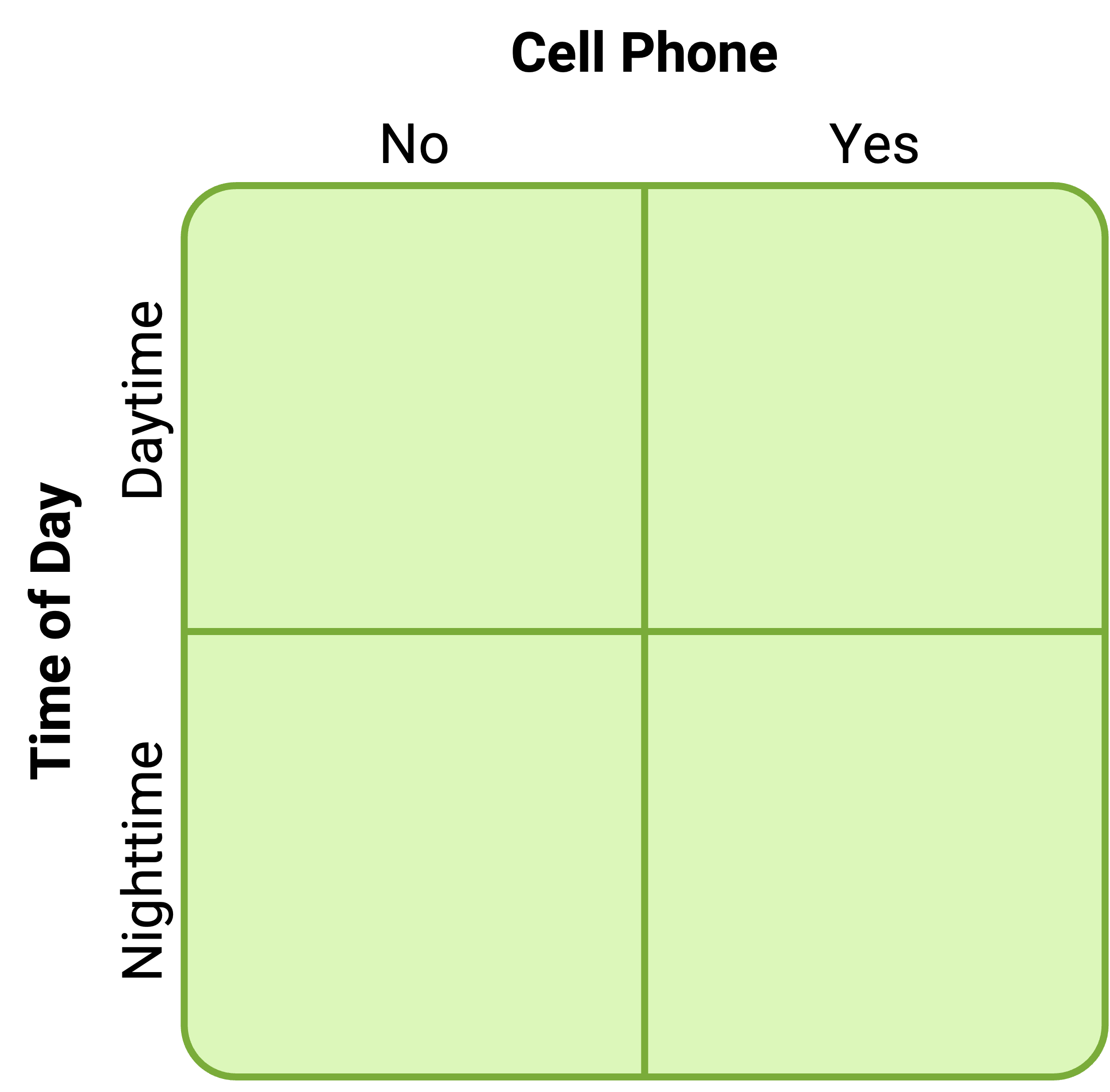
Figure 6.1: Factorial design table representing a 2 x 2 factorial design.
In principle, factorial designs can include any number of independent variables with any number of levels. For example, an experiment could include the type of psychotherapy (cognitive vs. behavioral), the length of the psychotherapy (2 weeks vs. 2 months), and the sex assigned at birth of the psychotherapist (female vs. male). This would be a 2 × 2 × 2 factorial design and would have eight conditions. Figure 6.2 shows one way to represent this design. In practice, these types of designs can have difficult to interpret effects. We will cover interactions later on in this chapter. As the complexity of the design increases it becomes hard to scale the logic of interaction effects for multiple variables. Even for this “simple” case of 2 x 2 x 2, it becomes hard to describe interactions if they occur. In practice, it is unusual for there to be more than three independent variables with more than two or three levels each because the number of conditions can quickly become unmanageable. For example, adding a fourth independent variable with three levels (e.g., therapist experience: low vs. medium vs. high) to the current example would make it a 2 × 2 × 2 × 3 factorial design with 24 distinct conditions. In the rest of this section, we will focus on designs with two independent variables with two levels. The general principles discussed here extend to more complex factorial designs, however, comparisons become very unwieldy when considering many factors, levels and their interactions.
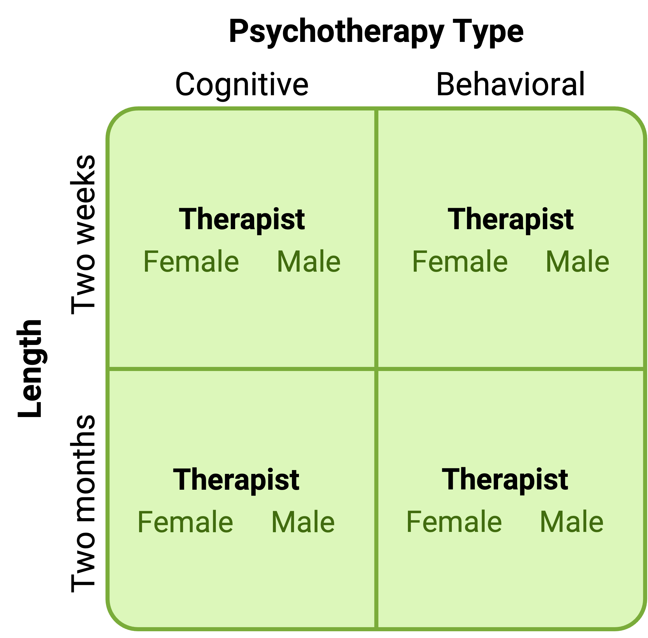
Figure 6.2: Factorial design table representing a 2 x 2 x 2 factorial design.
Assigning Participants to Conditions
Recall that in a simple between-subjects design, each participant is tested in only one condition. In a simple within-subjects design, each participant is tested in all conditions. In a factorial experiment, the decision to take the between-subjects or within-subjects approach must be made separately for each independent variable. In a between-subjects factorial design, all of the independent variables are manipulated between subjects. For example, all participants could be tested either while using a cell phone or while not using a cell phone and either during the day or during the night. This would mean that each participant was tested in one and only one condition. In a within-subjects factorial design, all of the independent variables are manipulated within subjects. All participants could be tested both while using a cell phone and while not using a cell phone and both during the day and during the night. This would mean that each participant was tested in all conditions. The advantages and disadvantages of these two approaches are the same as those discussed in the chapter on experimental research. The between-subjects design is conceptually simpler, avoids carryover effects, and minimizes the time and effort of each participant. The within-subjects design is more efficient for the researcher and controls extraneous participant variables.
It is also possible to manipulate one independent variable between subjects and another within subjects. This is called a mixed factorial design. For example, a researcher might choose to treat cell phone use as a within-subjects factor by testing the same participants both while using a cell phone and while not using a cell phone (while counterbalancing the order of these two conditions). But he or she might choose to treat time of day as a between-subjects factor by testing each participant either during the day or during the night (perhaps because this only requires them to come in for testing once). Thus each participant in this mixed design would be tested in two of the four conditions.
Regardless of whether the design is between subjects, within subjects, or mixed, the actual assignment of participants to conditions or orders of conditions is typically done randomly.
Nonmanipulated Independent Variables
In some factorial designs, one of the independent variables is a nonmanipulated independent variable. An example of this is a study by Halle Brown and colleagues in which participants were exposed to several words that they were later asked to recall (H. D. Brown et al., 1999). The manipulated independent variable was the type of word. Some were negative health-related words (e.g., tumor, coronary), and others were not health related (e.g., election, geometry). The nonmanipulated independent variable was whether participants were high or low in hypochondriasis (excessive concern with ordinary bodily symptoms). The result of this study was that the participants high in hypochondriasis were better than those low in hypochondriasis at recalling the health-related words, but they were no better at recalling the non-health-related words.
These types of designs may be common, but there are a couple drawbacks to using them. While they are still considered experimental as long as at least one independent variable is manipulated, regardless of how many nonmanipulated independent variables are included. However, it is important to remember that causal conclusions can only be drawn about the manipulated independent variable. Thus, in the previous example, we would not be able to infer causal evidence that people with high hypochondriasis causes more greater recall of health-related words. This evidence is the equivalent of correlation evidence. Thus it is important to be aware of which variables in a study are manipulated and which are not.
Graphing the Results of Factorial Experiments
The results of factorial experiments with two independent variables can be graphed by representing one independent variable on the x-axis and representing the other by using different kinds of bars or lines. (The y-axis is always reserved for the dependent variable.) Figure 6.3 shows results for two hypothetical factorial experiments. The top panel shows the results of a 2 × 2 design. Time of day (day vs. night) is represented by different locations on the x-axis, and cell phone use (no vs. yes) is represented by different-colored bars. (It would also be possible to represent cell phone use on the x-axis and time of day as different-colored bars. The choice comes down to which way seems to communicate the results most clearly.) The bottom panel of Figure 6.3 shows the results of a 4 × 2 design in which one of the variables is quantitative. This variable, psychotherapy length, is represented along the x-axis, and the other variable (psychotherapy type) is represented by differently formatted lines. This is a line graph rather than a bar graph because the variable on the x-axis is quantitative with a small number of distinct levels.
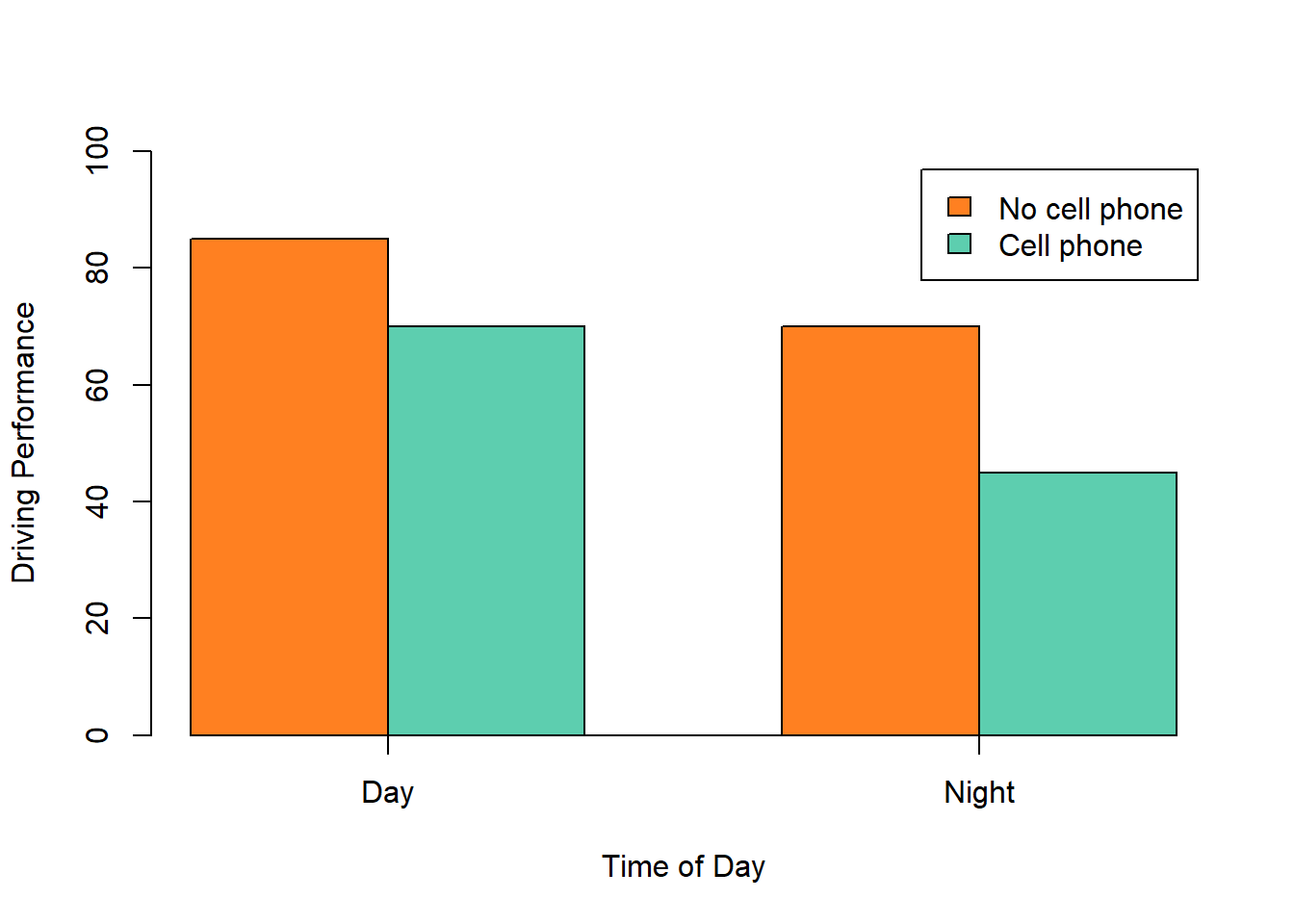
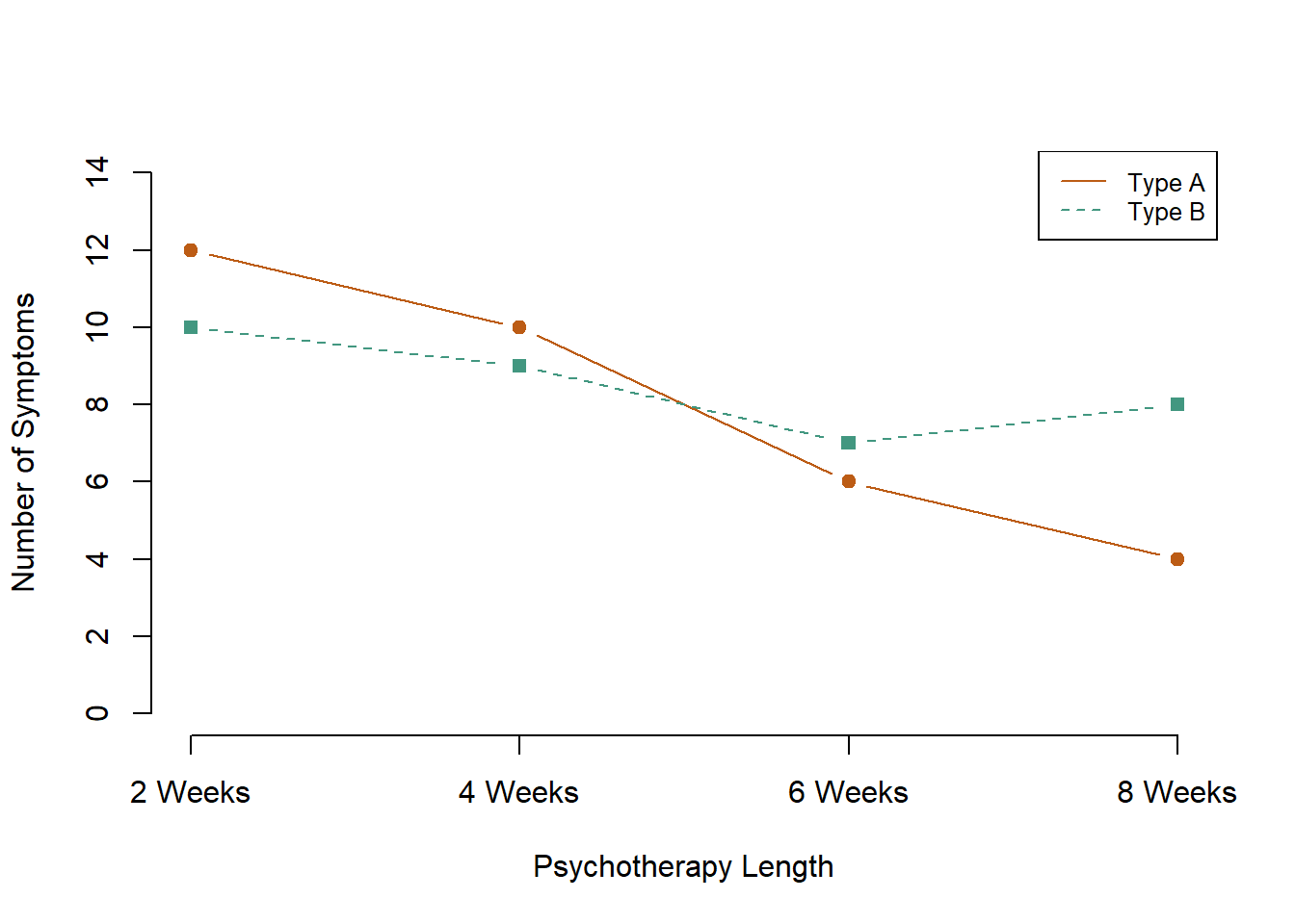
Figure 6.3: Two ways to plot the results of a factorial experiment with two independent variables.
Main Effects and Interactions
In factorial designs, we examine two key types of results: main effects and interactions (which are also called just “interactions”). A main effect shows the statistical relationship between one independent variable and a dependent variable, regardless of the levels of the other independent variable. Thus there is one main effect to consider for each independent variable in the study. The top panel of Figure 6.3 shows a main effect of cell phone use because driving performance was better, on average, when participants were not using cell phones than when they were. The blue bars are, on average, higher than the red bars. It also shows a main effect of time of day because driving performance was better during the day than during the night—both when participants were using cell phones and when they were not. Main effects are independent of each other in the sense that whether or not there is a main effect of one independent variable says nothing about whether or not there is a main effect of the other. The bottom panel of Figure 6.3, for example, shows a clear main effect of psychotherapy length. The longer the psychotherapy, the better it worked. But it also shows no overall advantage of one type of psychotherapy over the other.
There is an interaction effect (or just “interaction”) when the effect of one independent variable depends on the level of another. Although this might seem complicated, you have an intuitive understanding of interactions already. It probably would not surprise you, for example, to hear that the effect of receiving psychotherapy is stronger among people who are highly motivated to change than among people who are not motivated to change. This is an interaction because the effect of one independent variable (whether or not one receives psychotherapy) depends on the level of another (motivation to change). Schnall and her colleagues also demonstrated an interaction because the effect of whether the room was clean or messy on participants’ moral judgments depended on whether the participants were low or high in private body consciousness. If they were high in private body consciousness, then those in the messy room made harsher judgments. If they were low in private body consciousness, then whether the room was clean or messy did not matter.
The effect of one independent variable can depend on the level of the other in different ways. This is shown in Figures 6.4, 6.5, and 6.6. In 6.4, one independent variable has an effect at one level of the second independent variable but no effect at the others. (This is much like the study of Schnall and her colleagues where there was an effect of disgust for those high in private body consciousness but not for those low in private body consciousness.) In 6.5, one independent variable has a stronger effect at one level of the second independent variable than at the other level. This is like the hypothetical driving example where there was a stronger effect of using a cell phone at night than during the day. In 6.6, one independent variable again has an effect at both levels of the second independent variable, but the effects are in opposite directions. Figure 6.6 shows the strongest form of this kind of interaction, called a crossover interaction. One example of a crossover interaction comes from a study by Kathy Gilliland on the effect of caffeine on the verbal test scores of introverts and extroverts (Gilliland, 1980). Introverts perform better than extroverts when they have not ingested any caffeine. But extroverts perform better than introverts when they have ingested 4 mg of caffeine per kilogram of body weight. Figure 6.7, 6.8, and 6.9 shows examples of these same kinds of interactions when one of the independent variables is quantitative and the results are plotted in a line graph. Note that in a crossover interaction, the two lines literally “cross over” each other.

Figure 6.4: This bargraph is showing one of three types of interactions.This one shows that one independent variable has an effect at one level of the second independent variable but not at the other.
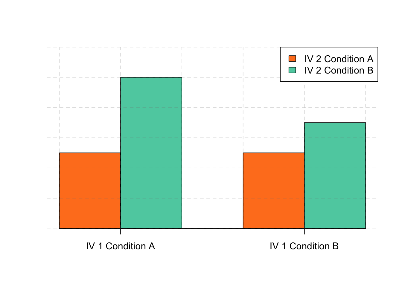
Figure 6.5: This bargraph is showing one of three types of interactions.This one shows that one independent variable has a stronger effect at one level of the second independent variable than at the other.
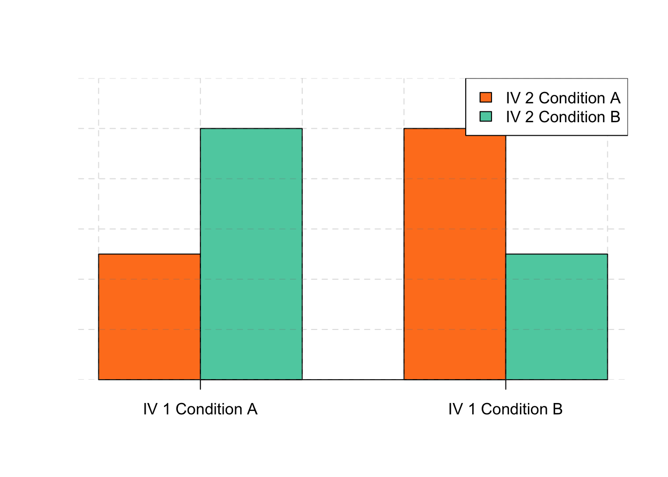
Figure 6.6: This bargraph is showing one of three types of interactions.This one shows that one independent variable has the opposite effect at one level of the second independent variable than at the other.
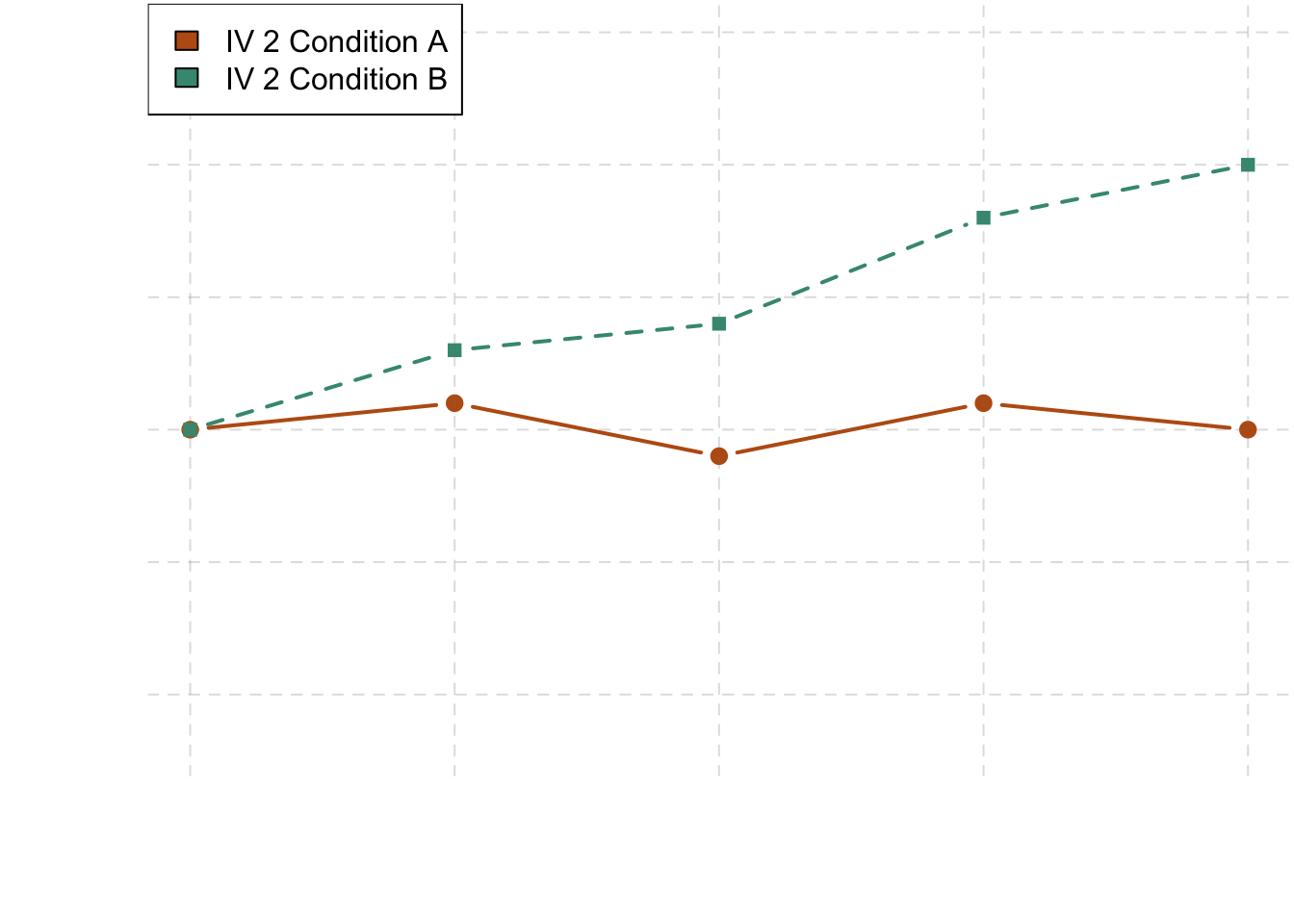
Figure 6.7: This linegraph is showing one of three types of interactions. This one shows that one independent variable has an effect at one level of the second independent variable but not at the other.
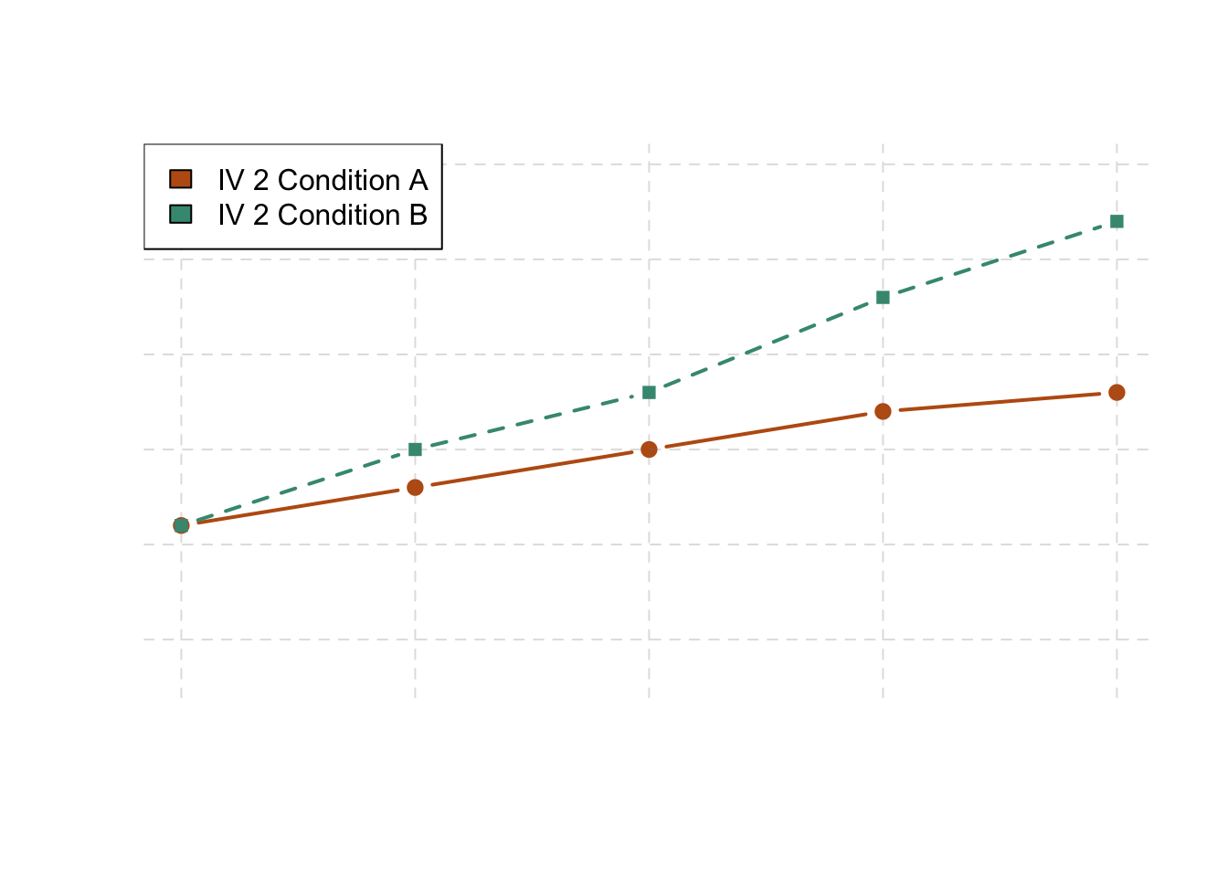
Figure 6.8: This linegraph is showing one of three types of interactions. This one shows that one independent variable has a stronger effect at one level of the second independent variable than at the other.
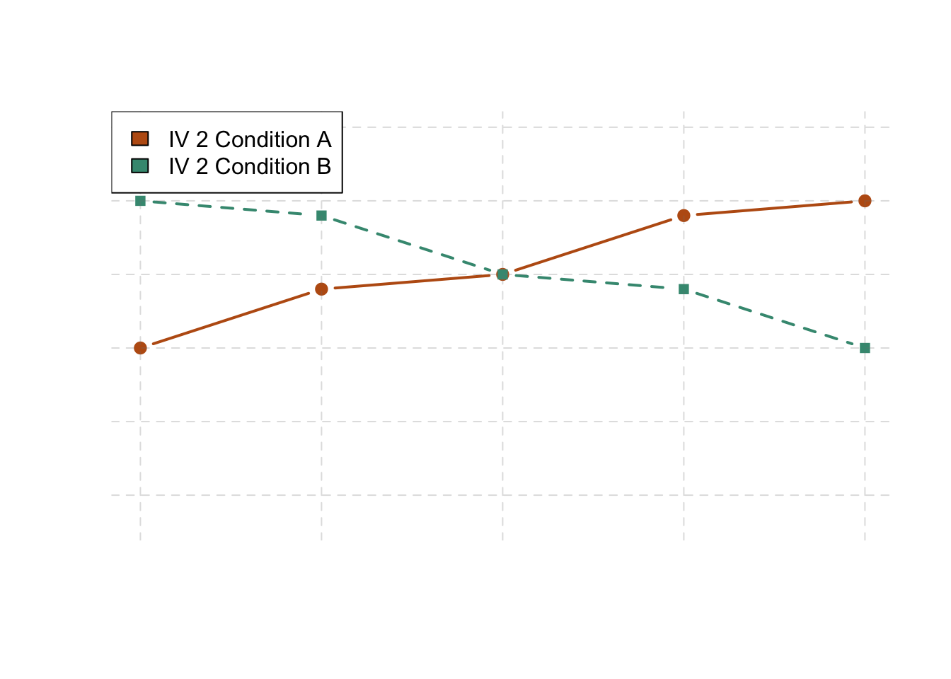
Figure 6.9: This linegraph is showing one of three types of interactions. This one shows that one independent variable has the opposite effect at one level of the second independent variable than at the other.
In many studies, the primary research question is about an interaction. The study by Brown and her colleagues was inspired by the idea that people with hypochondriasis are especially attentive to any negative health-related information. This led to the hypothesis that people high in hypochondriasis would recall negative health-related words more accurately than people low in hypochondriasis but recall non-health-related words about the same as people low in hypochondriasis. And of course this is exactly what happened in this study.
KEY TAKEAWAYS
- Researchers often include multiple independent variables in their experiments. The most common approach is the factorial design, in which each level of one independent variable is combined with each level of the others to create all possible conditions.
- The main effect of an independent variable, in a factorial design, is its overall effect averaged across all other independent variables. There is one main effect for each independent variable.
- Interaction effects between two independent variables is when the effect of one depends on the level of the other.
EXERCISES
- Practice: Return to the five article titles presented at the beginning of this section. For each one, identify the independent variables and the dependent variable.
- Practice: Create a factorial design table for an experiment on the effects of room temperature and noise level on performance on the SAT. Be sure to indicate whether each independent variable will be manipulated between subjects or within subjects and explain why.
6.3 Glossary
between-subjects factorial design
A factorial design in which each independent variable is manipulated between subjects so that each participant is tested in only one condition.
crossover interaction
An interaction in which one independent variable has opposite effects at different levels of another independent variable.
factor
An independent variable in a factorial design. Also in factor analysis, one of the underlying constructs that is assumed to account for correlations among multiple variables.
factorial design
A research design with multiple independent variables in which each level of one independent variable is combined with each level of the others to produce all possible conditions.
factorial design table
A table used to represent a factorial design. The rows represent the levels of one independent variable, the columns represent the levels of a second independent variable, and each cell represents a condition.
interaction
In a factorial design, when the effect of one independent variable depends on the level of another independent variable.
main effect
In a factorial design, the effect of one independent variable averaged across levels of all other independent variables.
mixed factorial design
A factorial design in which at least one independent variable is manipulated between subjects and at least one is manipulated within subjects.
multiple dependent variables
More than one dependent variable in the same study. They can be measures of different variables, including a manipulation check, or different measures of the same construct.